Distilling a 108K-parameter multi-agent policy into 1.4K parameters
I distilled a recurrent multi-agent policy from 107,721 actor parameters to 1,377 parameters without reducing its score on a sampled 20-episode evaluation. The result repeated across three student initializations using the same teacher and dataset.
This is evidence that a very small actor can represent behavior with comparable task performance under this evaluation protocol. It is not evidence that the student learned exactly the same policy, that 1,377 parameters is the minimum possible size in this setup, or that RL can train this architecture from scratch.
The experiment came from some of my ongoing work on communication in multi-agent RL. Before attributing performance differences to communication or a training algorithm, I wanted to test a simpler possibility: was the actor architecture itself too small to represent a good policy?
Experimental setup
The task is a 20-agent PettingZoo Pursuit environment. Twenty pursuers coordinate to capture eight evaders on a $40\times40$ grid. Each episode lasts at most 500 steps.
The teacher is a recurrent transformer actor trained with multi-agent PPO (MAPPO). It has 107,721 parameters and captured all eight evaders in each of the 20 sampled evaluation episodes used here.
Two metrics are reported:
- Catch%: the number of captured evaders divided by eight, averaged over episodes.
- Done%: the percentage of episodes in which all eight evaders were captured.
The actor receives a local observation at each step and maintains a GRU hidden state. In the equations below, $s_t$ means the information available to the actor at time $t$: the current observation together with the recurrent state produced by the previous observation history.
The question is:
How small can this actor become while retaining comparable task performance under the same evaluation protocol?
This is different from asking whether RL can train the small actor from scratch. Distillation tests whether supervised optimization can find a small policy with the desired behavior. It does not test whether reward-driven exploration can find that policy.
Imitation learning, behavioral cloning, and distillation
Imitation learning is the general problem of learning behavior from an expert rather than directly from reward. The methods differ along two independent axes.
The first axis is the target.
- A hard target records one expert action and trains with ordinary cross-entropy.
- A soft target records the expert's complete action distribution and trains against that distribution.
The second axis is the source of training states.
- Offline methods use a fixed dataset, usually collected from the expert.
- Interactive methods collect states from the learner while an expert supplies labels.
These choices produce four useful cases:
| Hard action target | Full distribution target | |
|---|---|---|
| Fixed expert trajectories | Behavioral cloning | Offline policy distillation used in Stage A |
| Learner-generated trajectories | Classic DAgger | DAgger-style policy distillation used in Stage B |
Inverse RL and adversarial imitation learning address related problems but use different supervision. Inverse RL infers a reward or cost that explains expert behavior. GAIL uses an adversarial objective to match the learner's state-action occupancy to the expert's occupancy. These methods are useful when expert trajectories are available but the expert's internal action probabilities are not. In this experiment I own the teacher network and can query its complete action distribution, so direct policy distillation is simpler.
Same per-state loss, different training states
Both stages use the forward KL divergence from the teacher distribution to the student distribution:
$$ \mathrm{KL}\left(\pi_T(\cdot\mid s),\Vert,\pi_\theta(\cdot\mid s)\right) = \sum_a \pi_T(a\mid s)\log\frac{\pi_T(a\mid s)}{\pi_\theta(a\mid s)}. $$
Stage A averages this loss over a fixed dataset of teacher trajectories:
$$ \min_\theta;\mathbb E_{s\sim d_T} \left[\mathrm{KL}\left(\pi_T(\cdot\mid s),\Vert,\pi_\theta(\cdot\mid s)\right)\right]. $$
Stage B lets the student act, asks the teacher to label the visited states, and trains on a capped buffer containing trajectories from several student iterations. Its training distribution is therefore a mixture of the state distributions induced by those students, not only the final $d_\theta$.
This distinction matters because a small error changes the learner's next observation. Repeated errors can move the learner into states that were rare in the expert dataset. Let $T$ be the episode horizon and let $\varepsilon$ bound the learner's per-step classification error on expert-trajectory states. In the worst case, the probability of at least one error by step $t$ is at most $\min(1,t\varepsilon)$; summing this exposure over the episode produces the $O(T^2\varepsilon)$ behavioral-cloning bound. This result does not assume independent errors; the short union-bound proof is included in the appendix. Ross et al. show that, under their reduction and no-regret assumptions, interactive imitation can instead obtain a linear dependence of $O(T\varepsilon)$ when the error is measured on the state distributions induced during learning.
The practical rule is to start with offline distillation and add interactive collection only when the offline student appears to fail because of distribution shift.
Failure mode 1: evaluating a stochastic policy greedily
The teacher captured all evaders in 20 out of 20 episodes when actions were sampled from its categorical distribution. Greedy argmax evaluation captured only about 35% of the evaders under the same environment protocol.
A quick inspection of the rollouts suggested a coordination failure. Several pursuers can produce similar action distributions in symmetric situations. Argmax selects the same action for each of them, which can make them clump or repeat the same motion. Independent sampling breaks these ties. This is a hypothesis about the mechanism, not a controlled causal result; an evaluation-temperature sweep would test it more directly.
Parallel and autoregressive action selection
MAPPO is usually described using centralized training and decentralized execution: a centralized critic can use joint information to estimate value and produce the advantage signal used to train the actor, but the critic is removed during execution. The actor can share one set of parameters across every agent while still producing different distributions from their different observations and recurrent states. Decentralized execution, parameter sharing, and parallel action generation are separate choices: the first specifies what information an actor may use, while the last specifies whether current actions are selected simultaneously. Here the shared transformer processes the agent features in one batched pass and emits one categorical distribution per pursuer; all actions are then sampled simultaneously, with no action conditioned on another agent's action from the same step.
An autoregressive alternative would choose an agent order and condition each action on the actions already selected for that step. This can represent explicit same-step dependencies and break symmetric choices, but there is often no natural agent order, and sequential decoding makes latency grow with the number of agents unless agents are grouped or the dependency is approximated. Pursuit accepts simultaneous actions, so parallel generation matches the environment interface and is cheaper to execute. Given this shared, parallel action path, similar distributions in symmetric situations became a reasonable explanation for why independent sampling succeeds while greedy selection does not (which can obviously be verified from the setup)
Two decisions follow from the observation:
- Evaluate the teacher and student by sampling, because that is how the working policy acts.
- Train against the complete teacher distribution instead of replacing it with the teacher's argmax.
A hard-label distillation baseline is still needed to measure the second effect directly. The current experiment establishes that sampled soft-target students work; it does not isolate how much of the result comes from soft targets rather than sampled data collection.
Why forward KL preserves the soft target
For teacher distribution $p$ and student distribution $q$,
$$ \mathrm{KL}(p\Vert q) = \sum_a p(a)\log p(a)-\sum_a p(a)\log q(a) = H(p,q)-H(p). $$
$H(p)$ is constant with respect to the student. Minimizing forward KL is therefore equivalent to minimizing the soft cross-entropy
$$ -\sum_a p(a)\log q(a). $$
Every teacher action probability contributes to the gradient. A hard target instead minimizes $-\log q(\arg\max p)$ and discards all non-maximal probabilities.
A quick note on forward and reverse KL
Reverse KL uses $\mathrm{KL}(q\Vert p)$. Forward KL penalizes the student when it assigns too little probability to actions supported by the teacher. Reverse KL penalizes the student when it assigns probability to actions that the teacher considers unlikely. Under limited capacity, this difference often gives forward KL a mass-covering tendency and reverse KL a mode-seeking tendency.
That general distinction is relevant here because the teacher relies on stochastic action selection. It does not prove that reverse KL would reproduce the greedy failure; that would require a direct comparison. Forward KL is used because it is exactly the soft-target cross-entropy for the available teacher probabilities.
The standard distillation temperature $T$ can soften both distributions, with the soft-target loss commonly scaled by $T^2$ as described by in the original distillation paper. All reported runs here use $T=1$. Temperature was not ablated during training.
Exposing complete action probabilities
The normal actor interface samples an action and returns the probability of that selected action. Distillation needs the complete categorical distribution. The required hook follows the same actor path but returns normalized log probabilities for every action.
The code below is a simplified reference implementation. The transformer reshape is needed because attention operates across the agent dimension.
def forward_log_probs(self, obs, rnn_state, masks, available_actions=None):
obs =.**self
rnn_state =.**self
masks =.**self
rows = obs.shape[0]
if self.use_transformer:
# rows = batch_size * number_of_agents
obs_by_agent = obs.
// self self -1
features = self.. -1
else:
features = self.
features, rnn_state = self.
distribution = self.
# Categorical.logits is normalized log probability.
return distribution.logits, rnn_stateThe teacher uses this method to produce targets. The student uses it as its trainable forward pass. Both actors use the same five-action output space, while the student's transformer width, depth, and GRU width can be reduced independently of the teacher.
Stage A: collect a fixed teacher dataset
I sampled the teacher through the environment and stored complete episodes of (observation, teacher_log_probability) pairs. Complete episodes are needed because the student is recurrent.
with torch.:
teacher_logp, next_teacher_rnn = teacher.
action = torch.distributions.
logits=
.
# Store the full five-action target before stepping the environment.
episode_obs.
episode_teacher_logp.
The dataset contains 600 episodes and 3,067,600 agent-steps. The mean episode length is 255.63 steps, with a range of 58 to 500. Teacher log probabilities were stored as float16 to reduce storage. I did not run a precision ablation here, so it would be an interesting future experiment to see how resilient KL is to loss of precision.
Failure mode 2: treating a recurrent student as independent samples
At deployment, the student begins an episode with hidden state zero and updates that state at every step. Training on randomly shuffled individual timesteps would give the GRU a different input history from the one it receives during deployment.
I therefore train on complete episodes. Each episode starts with hidden state zero, shorter episodes are padded to the longest episode in the batch, and padded positions are excluded from the loss.
def masked_forward_kl(student_logq, teacher_logp, valid):
teacher_p = teacher_logp.
per_step = (
teacher_p * (teacher_logp - student_logq)
).dim=-1
return (per_step * valid). / valid..min=1
def train_episode_batch(student, optimizer, observations,
teacher_logp, valid, batch_episodes):
rnn = torch.
*
device=
masks = torch.
* *
1
device=
student_logq, _ = student.
loss =
optimizer.
loss.
torch.nn.utils. 1.0
optimizer.This sequence-consistent training avoids an obvious train-deployment mismatch. A shuffled-timestep baseline has not yet been run, so its quantitative effect remains a follow-up experiment.
Parameter sweep
Every student used the same dataset, a 90/10 episode split, Adam with learning rate $5\times10^{-4}$, batches of eight episodes, gradient clipping at 1.0, and 40 to 60 epochs. The smallest reported student used 60 epochs.
The evaluation used one sampled episode on each of 20 fixed environment seeds.
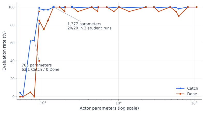
Selected results are below. “100” means all eight evaders were captured in all 20 evaluation episodes.
| Actor | Parameters | Catch% | Done% |
|---|---|---|---|
| Teacher, width 64 / 3 blocks | 107,721 | 100.0 | 100 |
| Student, width 48 / 2 blocks | 48,105 | 100.0 | 100 |
| Student, width 16 / 2 blocks | 6,953 | 100.0 | 100 |
| Student, width 8 / 2 blocks | 2,425 | 100.0 | 100 |
| Student, width 6 / 1 block / 2 heads | 1,377 | 100.0 | 100 |
| Student, width 4 / 1 block | 889 | 98.1 | 85 |
| Student, width 3 / 2 blocks | 765 | 63.1 | 0 |
| Student, width 2 / 1 block | 497 | 4.4 | 0 |
The 1,377-parameter configuration repeated the 20/20 result across three student initializations. The 889-parameter configuration was unstable as its three runs obtained Catch/Done scores of 98.1/85, 81.2/40, and 99.4/95.
Stage B: a DAgger-style control
I tested whether learner-generated states could recover the 765-parameter student. The student was initialized from its offline checkpoint, then trained for 15 rounds. Each round collected 48 episodes with the student acting and the teacher labeling every visited state. The aggregation buffer retained at most 600 recent episodes. The rollout mixture coefficient was $\beta=0$, so the student selected every environment action.
The offline student scored 63.1 Catch and 0 Done. After the DAgger-style stage it scored 66.9 Catch and 5 Done on the 20-episode sampled evaluation. Rollout Catch remained near 58–62% during training, and training KL remained near 0.50 instead of decreasing.
This control produced no convincing recovery. It makes distribution shift a less likely explanation for this particular failure, but hints at (without any empirical proof) 765 parameters being insufficient. The result could also be because of a number of reasons such as optimization difficulty, initialization or the chosen training schedule.
Reproducibility
The snippets above specify the method at the level needed to implement it in another policy framework. Reproducing the exact checkpoints additionally depends on the original framework implementation, initialization, collected trajectories.
| Component | Configuration |
|---|---|
| Environment | PettingZoo 1.26.1, Pursuit v4 |
| Task | 20 pursuers, 8 evaders, $40\times40$ grid, horizon 500 |
| Observation | 98 values per agent: $7\times7$ ally and opponent channels |
| Action space | Five discrete actions |
| Rewards | Catch 5.0, tag 0.0, urgency 0.0 |
| Teacher | Transformer width 64, 3 blocks, 4 heads, GRU width 64 |
| Teacher size | 107,721 actor parameters |
| Student | Transformer width 6, 1 block, 2 heads, GRU width 6 |
| Student size | 1,377 actor parameters |
| Dataset | 600 sampled teacher episodes; 3,067,600 agent-steps |
| Split | 540 training episodes; 60 validation episodes |
| Objective | Forward KL at temperature 1 |
| Optimizer | Adam, learning rate $5\times10^{-4}$ |
| Training | 60 epochs, 8 episodes per batch, gradient clipping at 1.0 |
| Student seeds | 1, 2, and 3 for the replicated 1,377-parameter result |
| Evaluation | One sampled episode on each of 20 fixed environment seeds |
The 1,377 parameters are distributed as follows:
| Student component | Parameters |
|---|---|
| Observation normalization and $98\rightarrow6$ projection | 790 |
| One transformer block | 276 |
| Transformer output normalization | 12 |
| GRU and recurrent normalization | 264 |
| $6\rightarrow5$ categorical action head | 35 |
| Total | 1,377 |
The current result motivates four direct experiments:
- Train a hard-label student on teacher argmax actions and compare it with the soft-target student.
- Evaluate several action-sampling temperatures and relate policy entropy to Catch and Done.
- Train the 1,377-parameter architecture from scratch with reinforcement learning.
- Compare recent methods for autoregressive language-model distillation, where the same training-generation mismatch appears:
- GKD trains on student-generated sequences labeled by the teacher. It is the closest language-model analogue to the DAgger-style stage used here.
- DistiLLM combines a skew KL objective with adaptive off-policy reuse of student-generated sequences, reducing the cost of fully on-policy collection.
- Speculative Knowledge Distillation lets the student propose tokens and lets the teacher replace proposals it ranks poorly. This interpolates between teacher-generated and student-generated trajectories.
- DistiLLM-2 uses different objectives for teacher- and student-generated responses, increasing the likelihood of teacher responses while decreasing the likelihood of student responses.
Appendix: the quadratic error bound
Let $E_i$ be the event that the learner makes an error at step $i$ while it is still following the expert trajectory, and assume $\Pr(E_i)\leq\varepsilon$. The event that at least one error has occurred by step $t$ is
$$ D_t = E_1\cup E_2\cup\cdots\cup E_t. $$
The union bound gives
$$ \Pr(D_t) \leq \sum_{i=1}^{t}\Pr(E_i) \leq t\varepsilon, $$
or more precisely $\Pr(D_t)\leq\min(1,t\varepsilon)$ because a probability cannot exceed one. This does not require the events $E_i$ to be independent. If they were independent and each had probability exactly $\varepsilon$, the probability would be $1-(1-\varepsilon)^t$, whose first-order approximation is $t\varepsilon$ when $t\varepsilon$ is small.
After the first error, the learner may enter states outside the expert's training distribution. Bounding the possible additional cost at step $t$ by $\Pr(D_t)$ and summing across the horizon gives
$$ \sum_{t=1}^{T}\Pr(D_t) \leq \sum_{t=1}^{T}t\varepsilon = \frac{T(T+1)}{2}\varepsilon = O(T^2\varepsilon). $$