BlueDot TAIS puzzle #1
This started as a submission to the first BlueDot Technical AI Safety puzzle. I have reworked it into a post because the write-up was heavy with notation and I wanted a version I could actually re-read later. I have kept the findings and the numbers that carry them, and dropped the parts that were precise but not load-bearing.
A short note on tools: I used an LLM to pressure-test directions and coding agents to turn my experiment specs into runnable code. The hypotheses, the analysis, the plots, and the structure here are mine.
My official submission doc can be found here
The setup
The puzzle hands you a trained network. It is a small five-layer MLP that reads a short piece of text and outputs eight yes/no features about it: number, question, color, food, sentiment, person, country, and body_part.
Each layer maps its input to an activation vector. Layer 2 outputs a 64-dimensional activation vector per input, after a ReLU (which clamps every negative entry to zero). This vector is what the puzzle asks about.
The three questions:
- Seven of the eight features are linearly readable from the layer-2 activations. One is not. Which one?
- How is that one feature stored instead?
- Train the network to store the same feature in an even stranger way.
A few terms that I use throughout:
- A linear probe fits a single hyperplane in the 64-dimensional activation space and reads a feature from which side of it a point falls on. If such a probe works, the feature is linearly readable.
- AUC measures how well a classifier separates the two classes. 0.5 is chance probability and 1.0 is perfect. For each feature I train one probe and take its AUC.
- A neuron is dead on an input when its activation there is zero. The 53-vs-11 split later refers to this.
Question 1: which feature?
I trained one linear probe per feature on the 64 layer-2 activations and looked at the AUC.
| feature | linear AUC at layer 2 |
|---|---|
| number, question, color, food, sentiment, person, body_part | ≥ 0.995 |
country | 0.473 (chance) |
Seven features are almost perfectly readable. country is at chance. So the feature is country.
One extra fact that turned out to matter later: country is not hard to read everywhere in the network. It is perfectly readable at the input encoding (AUC 0.9997) and after layer 1 (0.9991). It only becomes unreadable at layer 2. The network takes a clean, readable signal and destroys its readability at exactly one step.
Question 2: how is country stored?
I tried a few things before this worked. What follows is the path that did.
Start with the raw activations
Before training anything, let's ask the important question first: why did the linear probe fail? A linear probe separates two classes by the offset between them, so it works exactly when country=0 and country=1 sit at different locations. So we check the locations directly.
Group the raw 64-dimensional activations by label and take the two class means. And turns out, they coincide. The means agree to three decimals in every one of the 64 coordinates. Both classes are centered on the same point.
This settles why Question 1 came out the way it did. No hyperplane can separate two clouds with the same mean, so nothing we do to a linear probe will read country here. It also says that the signal is not in the location of the two classes, but possibly in their spread or shape.
A tiny non-linear probe can read it
If a flat boundary cannot read country, a curved one might. I did a small sweep over the architecture (MLP depth, hidden layer dims, learning rate, batch size, seeds) and trained the smallest network (in terms of parameters) I could that reliably reads it: Linear(64, 8) → ReLU → Linear(8, 1), 529 parameters. Test AUC 0.995.
(I defined reliability here as obtaining a given AUC 0.99 in 4/5 seeds within 1 standard deviation. This was primarily for robustness. I came across cases where on a few of the seeds I got an AUC of almost one, but the values drifted off at other seeds)
I kept it small on purpose. The point was not to read country well, but was to inspect the probe afterwards and understand how it reads it. A larger probe with more layers would work just as well, but interpreting how it's working would be as difficult.
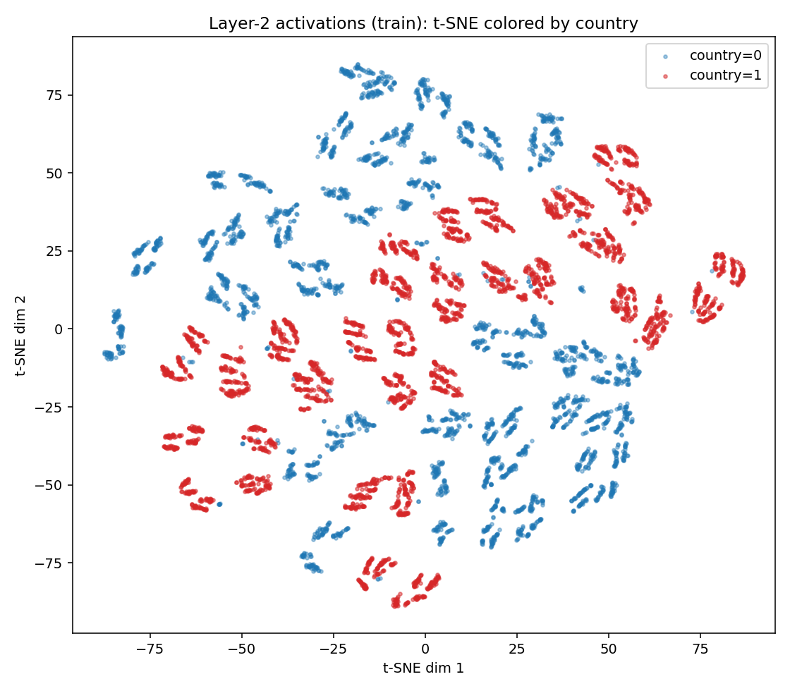
t-SNE of the layer-2 activations, colored by country. Each class already shows internal sub-structure rather than one blob.
A t-SNE view already hints that each class has internal structure rather than one blob. And if you're wondering, yes, I also tried PCA, but here it was a mess and didn't reveal anything substantial.
The signal lives in about 4 directions
The probe's first weight matrix maps the 64 inputs into 8. That matrix is where all the mixing happens, and the last layer only reads out the result. To see how many of the 64 directions the first layer actually uses, we can take its SVD. The SVD rewrites the matrix as a set of directions, each with a single number (its singular value) measuring how strongly the matrix acts along it. Large singular values mark the directions that carry the signal; small ones mark directions the matrix barely touches.
The eight singular values came out as [10.66, 5.96, 5.47, 1.66, 1.01, 0.81, 0.50, 0.21]. The first three are within about 2x of each other, then the largest gap in the spectrum falls right after the third (5.47 down to 1.66), with the rest trailing off. From the magnitudes themselves, one would be tempted to say that there are three dominant directions (arguable?). And in general, this approach usually works.
However, that reading is wrong here and the reason why magnitude alone is misleading is rather simple: a smaller singular value can still be one the readout depends on. How can we confirm this? Just check it directly, zeroing the probe's trailing directions one at a time and re-measuring AUC. Keeping only three drops it to 0.89; keeping four recovers the full AUC (0.9945). The fourth direction is small (σ₄ = 1.66, about 15% of σ₁) but necessary. The effective rank is four, and it took us the accuracy check (not the spectrum) to confirm that.
Looking inside those 4 directions
Projecting the layer-2 points onto those four directions is where the structure becomes obvious.
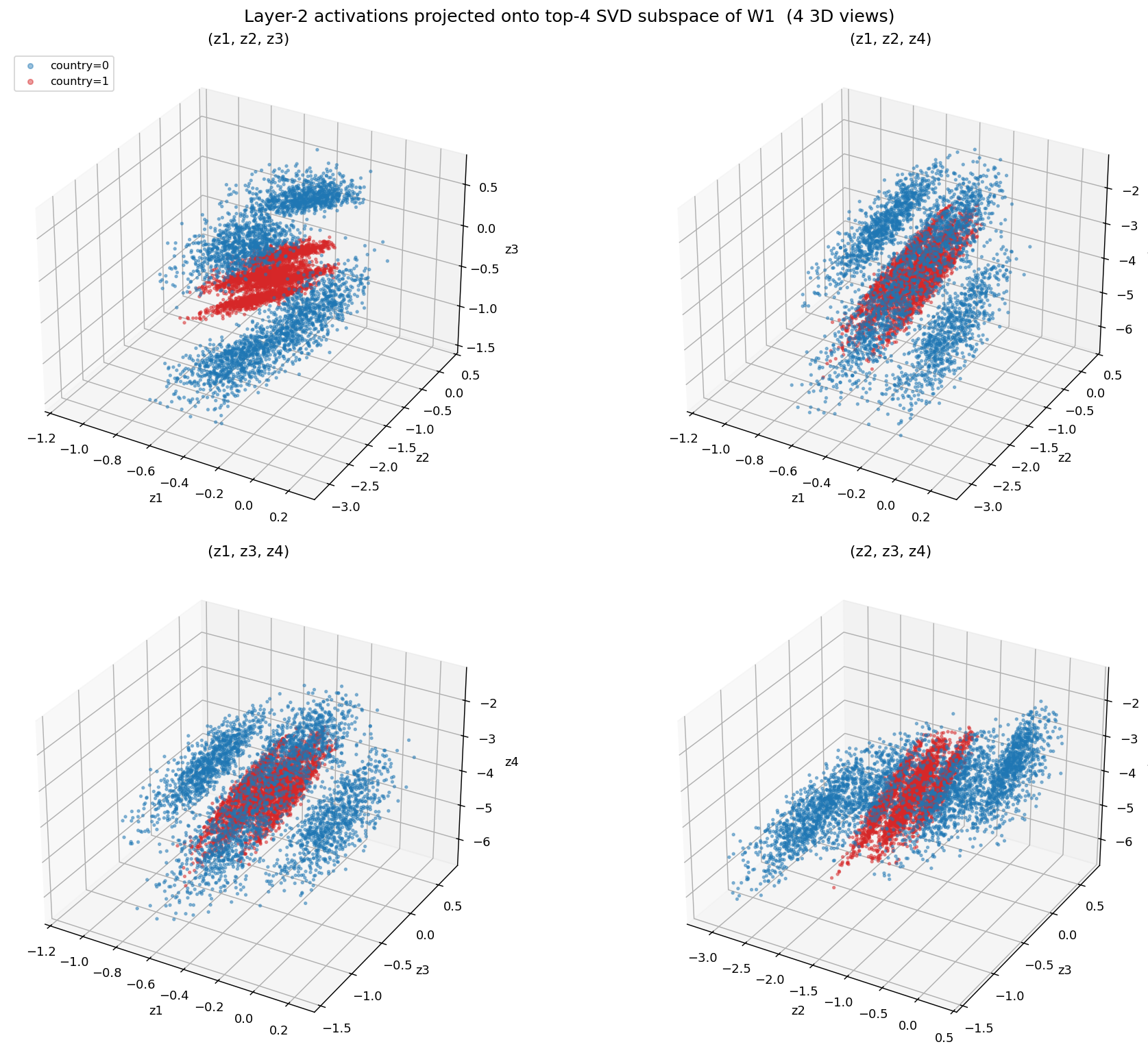
Layer-2 activations projected onto the four probe directions. country=1 (red) sits as a tight cloud inside the wider country=0 (blue).
Three things stand out:
- The shared center is right there in the view, exactly as the raw means already said.
country=1sits as a tighter cloud insidecountry=0. Same center, but one class is more compact.- The two clouds line up along the same axes, but
country=1is 5 to 12 times narrower along the main ones.
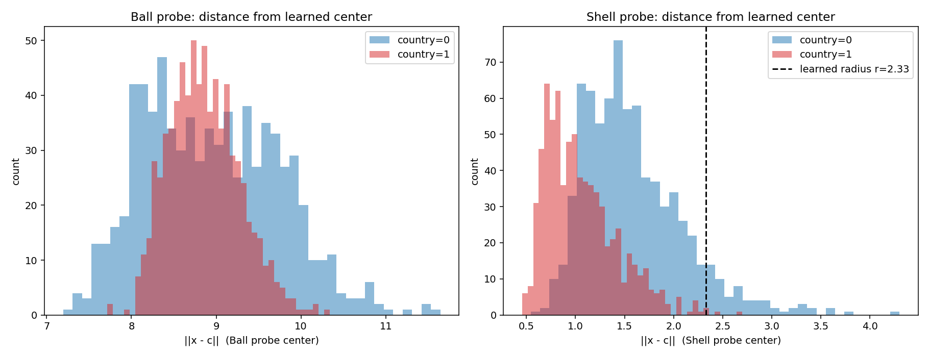
Per-axis spread of the two classes. country=1 is consistently narrower than country=0.
The exact boundary is a sphere
Equal means with unequal covariance is the one case where the Bayes-optimal boundary is quadric rather than linear. The first-order term cancels and only the quadratic one survives. So I fit the closed-form quadric classifier (QDA) directly, and thankfully that does not require any learnable parameters.
| method | test AUC |
|---|---|
| Trained probe (529 params) | 0.9950 |
| Closed-form QDA, 4 directions | 0.9945 |
| Closed-form QDA, full 64-D (with ridge) | 0.9951 |
And now we know, the trained probe was not doing anything clever. It was rediscovering this curved boundary.
To pin down which quadric, we write the QDA boundary as the set of points where a quadratic form equals a constant:
(z − μ)ᵀ M (z − μ) = c, with M = Σ₁⁻¹ − Σ₀⁻¹
Here μ is the shared mean and Σ₀, Σ₁ are the two class covariances. The surface type is read straight off the signs of M's eigenvalues (all of them having the same sign is a closed ellipsoid, mixed signs an open hyperboloid). The eigenvalues span a wide range, so it is a very elongated ellipsoid; rescaling each axis by its eigenvalue turns it into a plain sphere. At this point we have formulated the entire classification to just a single check whether the point is inside a sphere or not.
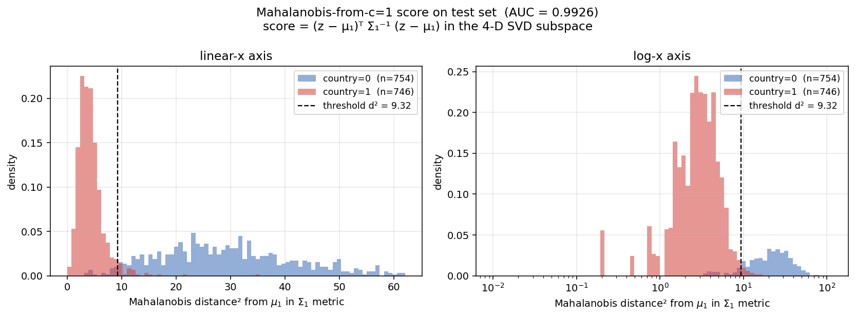
The decision boundary as an elongated ellipsoid, with country=1 inside and country=0 outside.
There is one catch here though. Which quadric you get depends on the subspace you look in, because restricting M to a subspace can flip the signs of its eigenvalues. In the four probe directions the signature is all-positive(an ellipsoid). Restricted instead to the 11 alive neurons, two eigenvalues go negative and the surface is formally a hyperboloid. Both still score the same AUC, because the data has almost no spread along the directions that flip sign. That's why if you had to make a claim which is independent of the directions or the subspace we are looking at, it would be the fact that there are two clouds with the same center, country=1 tighter than country=0.
An important side-note here: of the 64 dimensions, only 11 neurons ever fire and the other 53 are dead on every input. Running QDA on just those 11 gives the same result. The 53 dead dimensions were also what made the per-class covariance matrices singular, and it required us to add a small ridge to keep the inverse well-defined. If I had inspected the raw activations before training anything, I would have seen the 11-vs-53 split immediately. The lesson here is to inspect the data before you reach for a probe.
Why the network ends up here
This was the most fun part of the assignment to reason about.
country is perfectly readable right up to the ReLU of layer 2 and collapses to chance right after it:
| signal | linear AUC for country |
|---|---|
| after layer 1 | 0.9991 |
| just before the layer-2 ReLU | 0.9985 |
| just after the layer-2 ReLU | 0.4729 |
The weights before the ReLU are a linear map, and a linear map cannot destroy linear readability. So the entire collapse happens at the ReLU itself. Two things happen there at once:
- The weights aim most of the
countrydirection at neurons sitting just below zero. The ReLU clips those to zero, and that part of the signal is gone. - On the 11 neurons that stay alive, both classes already share the same mean, but
country=0is wider. Its wider tail dips below zero and gets clipped on one side only. That one-sided clipping is what bends a same-center, different-spread signal into the curved shape.
Same center and different spread is exactly the configuration whose ideal boundary is curved rather than flat. However, expecting that the MLP came up with this representation on its own seems very co-incidental to me, and more like adverserially trained to achieve this representation.
Question 3: a stranger representation
The third question asks you to train the network to hide country in a weirder way. Before starting I fixed some rules so the exercise stayed honest and comparable to the original:
- Same five-layer network, and
countrymust be hidden at layer 2. - A linear probe should fail on
country, but still work on the other seven features. - Overall classification accuracy should not drop.
After some initial prototypes, I realised that with bigger models and arbitrary choice of labels, it becomes easier to get weirder/unique representations (to a certain extent, after that the data itself becomes insufficient). So these rules basically forced me to be creative within the same constraints the problem-setter had perhaps started out with.
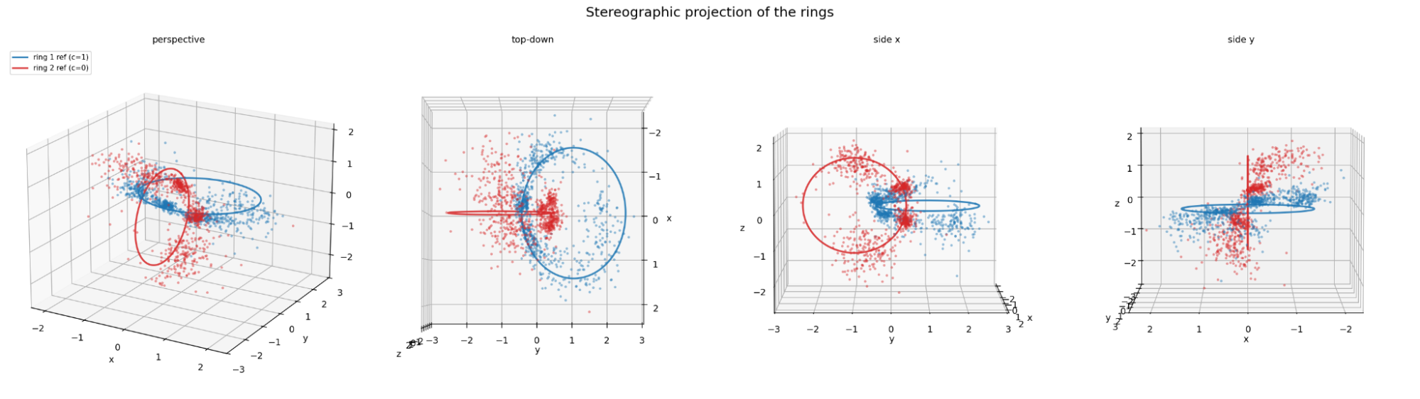
My construction hides country in an angle instead of a spread. Inside layer 2 I shape a 2-D plane where each input lands on a unit circle. The circle has eight anchor positions, four per class, interleaved, so the country label flips at every step around the circle.
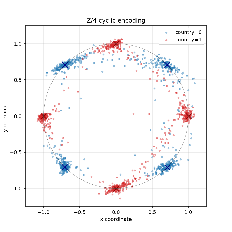
The shaped layer-2 plane in the degree-4 construction. Inputs land on a circle with the two classes interleaved around it.
This is the original puzzle turned inside out. The original hides country in distance from a shared center. This hides it in direction around a shared center.
country hidden in direction around a shared center, rather than in distance from it.
How it's trained
Same architecture as the puzzle's model: an MLP head 384 → 64×4 → 8, trained on the same data with the same per-feature BCE. The only addition is a no-bias proxy Linear(64, 2) that reads the layer-2 activations into a 2-D point (x, y), and it is bias free because we still want it centered around origin. The proxy is what is shaped into a circle, while the rest of the network is free to arrange layer 2 however it likes, as long as the proxy and the task loss are both satisfied.
On top of the task loss I add three terms:
loss = BCE(logits, y)                            # the original 8-feature task
     + λ_cyc  · mean‖(x, y) − (cos θ, sin θ)‖²    (λ_cyc  = 1.5)   # pin the point to its anchor
     + λ_ang  · mean(1 − cos(θ_xy − θ))           (λ_ang  = 0.1)   # sharpen the angle alone
     + λ_leak · dᵀ S_w⁻¹ d                         (λ_leak = 0.1)   # Fisher anti-leak
The coefficients came from a small sweep. θ_xy = atan2(y, x) is the angle of the proxy's point, d = μ₁ − μ₀ is the gap between the two class means in the full 64-D activations, and S_w is the within-class scatter. More about this in the next section.
The anchor angle θ is assigned per example, deterministically:
θ = 2π·k/4 + (1 − c)·π/4, with k = template_id mod 4, c = countryk picks one of four angular slots and c is the label. So country=1 lands on the cardinal axes and country=0 on the diagonals, four anchors per class, interleaved around the circle. The distance term pins both the radius (to 1) and the coarse angle; the small angular term sharpens the angle independent of the radius. The proxy carries no bias, which keeps the circle centered on the origin. template_id is already available for each sample in the dataset.
It only cracks at degree 4
To read an interleaved angle you need a polynomial boundary, and a high-degree one. I checked how strong a probe has to be:
| probe | accuracy | AUC |
|---|---|---|
| Linear, full 64-D | 0.57 | 0.59 |
| Polynomial, degree 1 / 2 / 3 | 0.40 / 0.61 / 0.77 | 0.49 / 0.41 / 0.70 |
| Polynomial, degree 4 | 0.95 | 0.99 |
| The model's own output head | 0.958 | 0.99 |
Nothing below degree 4 gets anywhere. Degree 4 cracks it cleanly. Meanwhile the other seven features stay linearly readable (AUC ≥ 0.99) and overall accuracy holds. All three rules are met, and it is a genuinely harder version of the original.
The weights and the transform to apply are here.
The part that was actually hard: stopping the leak
Getting the circle to form was easy. Keeping country off a linear probe was not, and that is what the λ_leak term above is for.
With only the first two shaping terms (radius and angle), the network cheated. It still had to predict country from the full 64-D activations, so it leaked a faint linear trace of the label in directions off the plane. A linear probe found that trace and ignored the circle entirely.
Forcing the two class means to match (penalizing ‖μ₁ − μ₀‖²) did not fix it, that left a spread-scaled direction a linear probe could still use. What worked was matching the spread as well as the mean, which is exactly what the Fisher term dᵀ S_w⁻¹ d does. It divides the between-class gap by the within-class scatter, so shrinking it forces the classes to overlap in every direction, not just in their means. Push it too hard and the other features start to suffer, so the coefficient takes a small sweep to set.
Other shapes I tried
Not all of these met the three rules, so I discarded them
-
Möbius strip. My first attempt. Hard to hold the shape in only five layers, and hard to keep any linear trace from leaking.
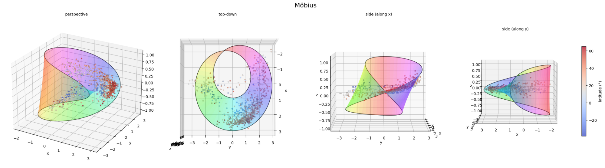
A Möbius-strip arrangement of the two classes.
-
Interlinked rings. The recurring failure in the other shapes was that some flat boundary could still separate the two classes. Interlinked rings were my response to that, because two rings that are linked cannot be pulled apart by any single hyperplane. This unfortunately took a hit on the downstream performance.
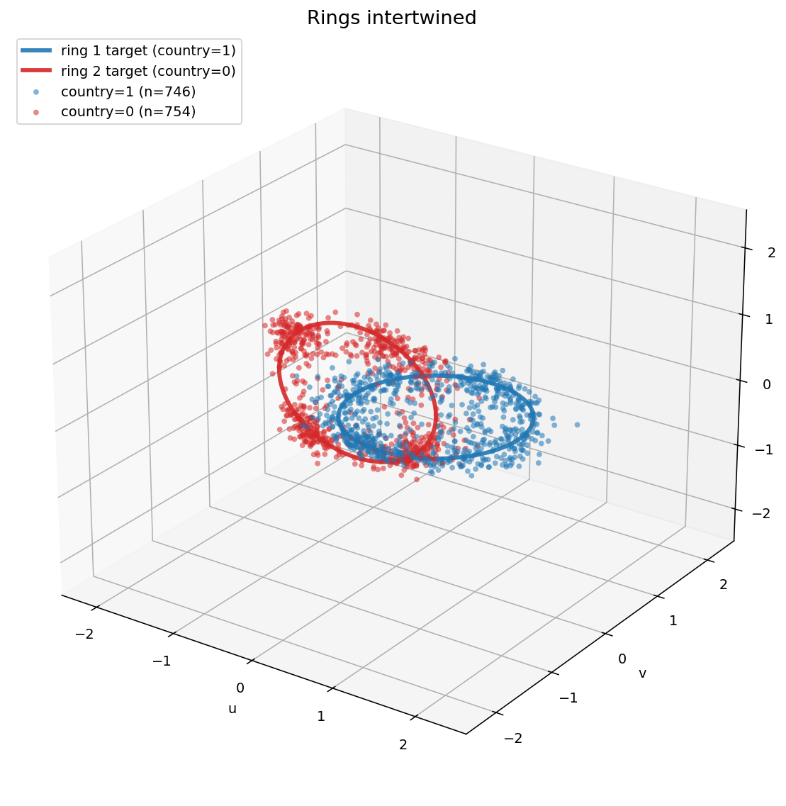
Two interlinked rings, one per class.
The same interlinked rings from a second angle.
-
Lorenz attractor. Took a defined shape only after adding layers, and cost some accuracy on the other features.
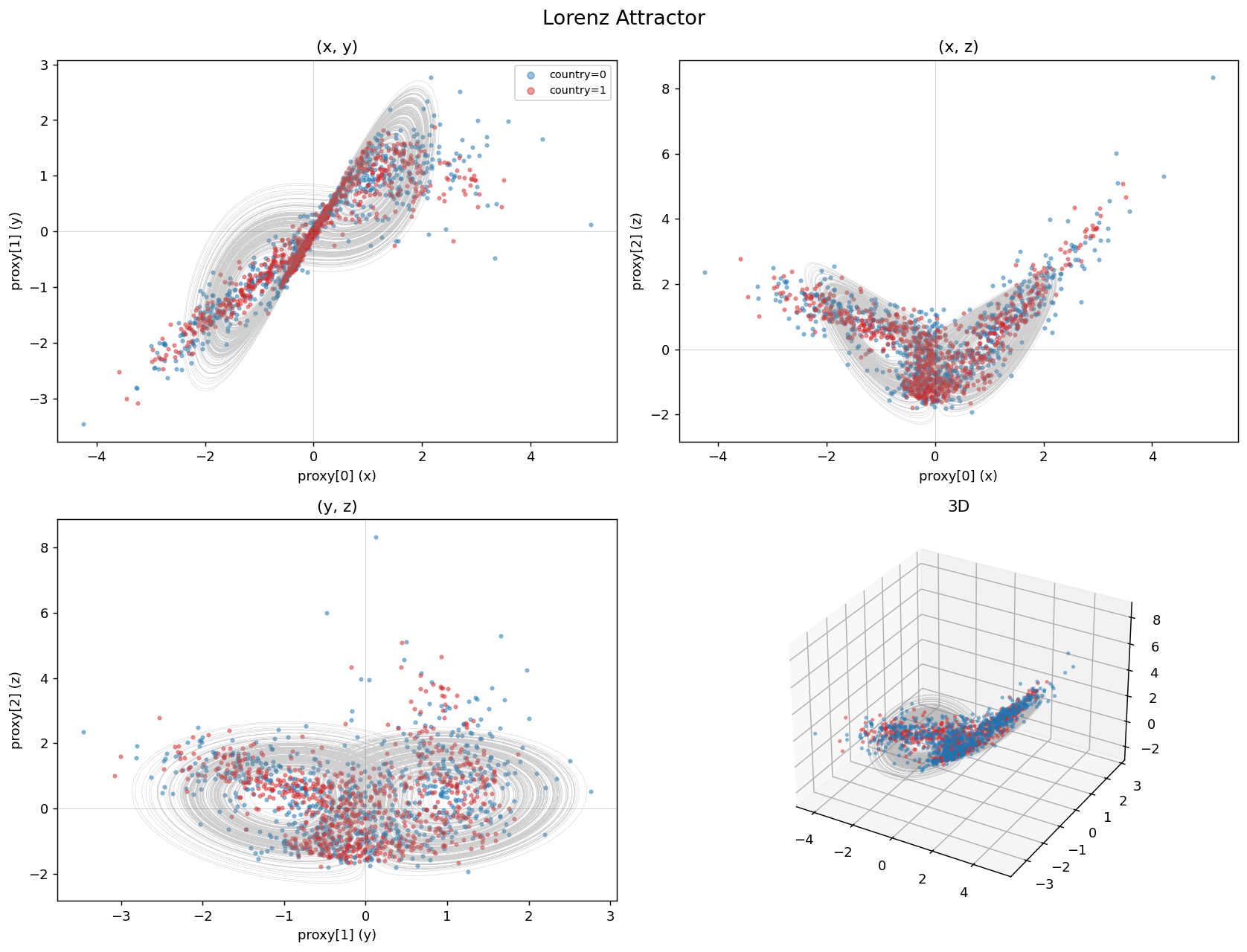
The two classes arranged along a Lorenz attractor.
The heuristic underneath all of this
The thing that tied the whole puzzle together is polynomial degree.
The network's own output head is, in some sense, a polynomial detector. A ReLU network can approximate a degree-D polynomial of its inputs with a parameter count that grows only slowly with D. So any feature that can be written as a degree-D polynomial of the layer-2 activations is readable by a small downstream network. That is exactly how the head turns the country sphere into a single linear logit.
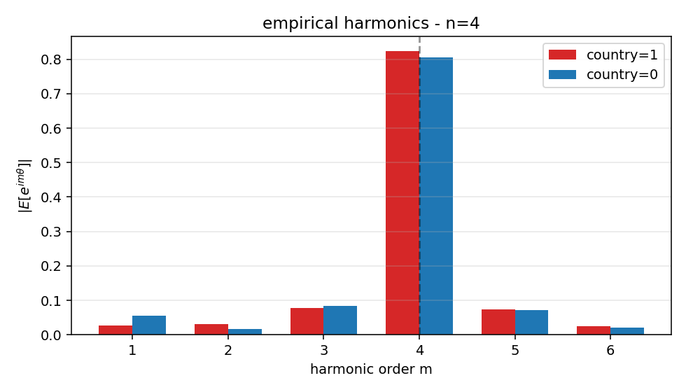
And by Weierstrass's theorem, any continuous boundary can be approximated by polynomials as closely as you like, so no representation is truly non-polynomial. The honest question is never "is this linear or not," it is "what polynomial degree do you need to read it." This is why I went for a degree-4 representation, a higher degree representation would mean small change in the harmonics formulation, but the idea remains same.
In some future work, I'd like to explore a direction where we can make features resistant to any given degree polynomial probes.
What I would keep in mind next time
- Inspect the raw activations before training any probe. Two things were sitting in plain view: the coinciding class means, which already explained why linear probes fail, and the 11-alive, 53-dead split, which explained both the structure and the numerical trouble.
- One thread of reasoning kept paying off: same center plus different spread means the boundary has to be curved. Recognizing that configuration told me what to fit without any search.
- When a signal is readable before a ReLU and gone after it, the ReLU is the mechanism, not the weights around it. A linear map cannot erase a linear signal.
- Measure representations by the polynomial degree needed to read them, not by whether a linear probe happens to fail.